← All tutorials

CAGrad (Conflict-Averse Gradient Descent)

Improve the task each step helps least, while still lowering the average loss.

On this page

1 What CAGrad does each step

A task’s loss measures how badly the model performs that task; its gradient points where that loss rises fastest, and training steps against it.

Each training step, CAGrad takes the gradient g_i of each task i over the shared weights, one entry per shared parameter, often millions (the figures draw two entries). It keeps training on the average loss and changes only the update’s direction, in three moves.

1. It searches a ball around the average gradient, the vectors within one radius of it. The radius is a set fraction of that gradient’s length, so the ball grows and shrinks with it (Section 2).
2. In the ball it looks for the update that most helps the least-helped task, the one whose loss drops least (Section 3).
3. That search comes down to choosing one weight per task, each zero or more and adding up to 1, so the least-helped task gains most. The weighted task gradients add up to the weighted gradient, and the update moves from the average gradient one radius along its direction (Section 4, Section 5).

CAGrad keeps no state between steps; the official CAGrad code restarts the weight solve from equal weights each step.

2 A ball around the average gradient

The average gradient g₀, the mean of the task gradients, can raise one task’s loss.

Searching only the ball around g₀ keeps the update near g₀, so the average loss still falls. ‖g₀‖ is the length of g₀. The hyperparameter c sets the radius as a fraction of that length, so the radius is c‖g₀‖.

At c = 0 CAGrad is plain gradient descent (GD); very large c gives the direction MGDA (Multiple Gradient Descent Algorithm) picks, the shortest weighted average of the task gradients. Raising c favors the least-helped task; lowering it stays near the average.

3 The worst-case improvement objective

A candidate direction d works like a gradient: parameters move against it.

4 Solving for one weight per task

A direction d has millions of entries, so CAGrad solves its dual problem instead: the same answer, found by searching over one weight per task. The weighted sum of the task gradients is the weighted gradient g_w.

G holds one task gradient per row. solve_weights takes the Gram matrix GG (the K×K table of dot products between task gradients) and c and returns w*.

import numpy as np
from scipy import optimize

def F(w, GG, c):
    g0_len = np.sqrt(GG.mean())
    center = w @ GG.mean(axis=1)
    gw_sq = max(w @ GG @ w, 0.0)
    gw_len = np.sqrt(gw_sq)
    ball = c * g0_len * gw_len
    return center + ball

CONSTRAINT = {"type": "eq", "fun": lambda w: w.sum() - 1}

def solve_weights(GG, c):
    K = len(GG)
    res = optimize.minimize(F, np.full(K, 1 / K), args=(GG, c), method="SLSQP",
                            bounds=[(0, 1)] * K, constraints=CONSTRAINT)
    return res.x

g1 = [3.0, 1.0]
g2 = [-1.0, 2.0]
G = np.array([g1, g2])  # (K, P)
c = 0.5
w_star = solve_weights(G @ G.T, c)

1. 1Computes F(w) from GG, lines 3 and 4 of the weight solve in Section 4; max stops rounding from going below zero.
2. 2Keeps the weights adding up to 1, the set Δ in line 2 of that solve.
3. 3Minimizes F from equal weights, each in [0, 1], the argmin in line 2.
4. 4Uses the two tasks of Figure 5 and returns w* = (0, 1).

5 The CAGrad update

Continuing from the solver of Section 4, this code turns w* into d*.

g_w = w_star @ G  # optimal g_w
g0 = G.mean(axis=0)
radius = c * np.linalg.norm(g0)
EPS = 1e-12  # zero-length guard
gw_len = np.linalg.norm(g_w)
unit = g_w / (gw_len + EPS)
d_star = g0 + radius * unit

1. 1Builds g_w* from w*, line 1 of the weight solve in Section 4.
2. 2The center g₀, line 1 of the update in Section 5, and the radius c‖g₀‖, line 2.
3. 3The fraction in line 2, guarded against length zero.
4. 4One radius out to d*, the best point in Figure 4.

6 One CAGrad update, step by step

7 Convergence guarantee

CAGrad provably reaches a stationary point of the average loss (zero gradient, possibly a saddle point), assuming H-Lipschitz gradients (the gradient changes at most H times as fast as the parameters), a loss bounded below, and step size α ≤ 1/H.

Take c = 0.5, the value in the worked example. The convergence bound has 1 − c² in its denominator, and 1 − 0.5² = 0.75 where plain gradient descent (c = 0) has 1. So CAGrad’s bound is 1 ÷ 0.75 = 1.333 times plain gradient descent’s.

1. Other proofs are weaker. MGDA proves only a Pareto-stationary end point; PCGrad, which removes the part of each task gradient that conflicts with another task’s, has a proof that covers two tasks with convex (bowl-shaped) losses.
2. At c of 1 or more, the guarantee is gone. The update can then settle where the average loss’s gradient is not zero, at a point that is only Pareto stationary.

8 Toy trajectories in loss space

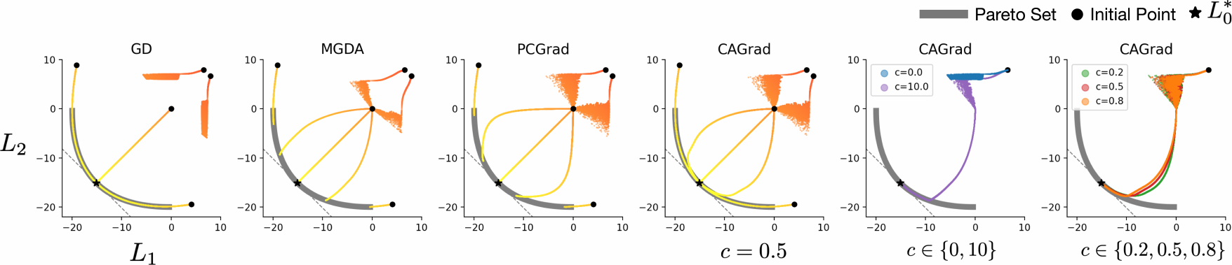
The paper’s toy has two parameters and two task losses, L₁ and L₂, run from five starts. Figures 7 to 9 plot loss space, one axis per task loss, with each start’s trail. The gray Pareto front holds the loss pairs where neither loss can drop without the other rising; the star is its lowest average loss.

Figure 7. Trails fade orange to yellow. GD stalls on 2 of 5 starts; MGDA stops where it first meets the front. Panels 1 and 2 of the paper’s Figure 3.

Figure 8. PCGrad also stops at the front; CAGrad, c = 0.5, takes all five to the star. Panels 3 and 4 of the paper’s Figure 3.

Figure 9. From one hard start, c = 0 stalls; c = 10 and 0.2 to 0.8 reach the star. Panels 5 and 6 of the paper’s Figure 3.

9 Six methods on the toy problem

The race in Figure 10 runs six methods on the paper’s toy code: each loss has a narrow curved valley in the upper half and a bowl in the lower half, with a ridge between. The Pareto set holds the parameters whose losses lie on the front.

All six use Adam (each parameter’s step scaled by its recent gradient size) for 60,000 steps. GradVac moves task gradients that agree less than usual toward a target angle. GradNorm reweights the task losses so they train at similar rates. The race runs the official toy code. That code divides CAGrad’s step by 1 + c, and one sign in its second loss differs from the formula printed in the paper.

10 Results over five starts

Of the two, only CAGrad has a convergence proof (Section 7). This GradNorm run is approximate, since GradNorm divides each loss by its starting value and these toy losses go below zero.

11 When to use CAGrad, and its cost

1. Use it when task gradients conflict and the average loss still matters.
2. Time per step is K backward passes plus the small solve. CAGrad-Fast keeps the guarantee while sampling a random task subset per step, 4 of 10 and 8 of 50 on Meta-World (Figure 12).
3. Memory holds K flattened shared gradients plus each task’s computation graph (what autograd keeps for a backward pass).

12 CAGrad in a PyTorch training step

The listing stacks the task gradients into G (Section 3 of Gradient Balancing Inside the Training Loop shows how each is computed), calls solve_weights (Section 4), and writes d* into the .grad of body, the shared backbone’s parameters. heads, each task’s output layers, get the average loss’s gradient.

import torch
from torch.nn.utils import clip_grad_norm_

c = 0.4  # radius c (NYUv2)
EPS = 1e-12  # zero-length guard

def flat_grad(loss, body):
    grads = torch.autograd.grad(loss, body, retain_graph=True)
    return torch.cat([g.ravel() for g in grads])

def fill_grads(params, vec):
    i = 0
    for p in params:
        n = p.numel()
        part = vec[i:i + n]
        p.grad = part.view_as(p)
        i += n

def cagrad(losses, parts, opt):
    body, heads = parts
    K = len(losses)
    rows = [flat_grad(L, body) for L in losses]
    G = torch.stack(rows)  # K x P
    GG = (G @ G.T).cpu().numpy()
    w_star = solve_weights(GG, c)
    w = torch.tensor(w_star).to(G)
    g0 = G.mean(dim=0)
    g_w = w @ G
    gw_len = g_w.norm()
    unit = g_w / (gw_len + EPS)
    radius = c * g0.norm()
    d_star = g0 + radius * unit
    opt.zero_grad()
    fill_grads(body, d_star)
    avg = sum(losses) / K
    avg.backward(inputs=heads)
    clip_grad_norm_(body + heads, max_norm=1.0)
    opt.step()

1. 1One task’s body gradient g_i, line 1 of the objective in Section 3, as one row of G.
2. 2Writes a flat vector into the .grad of body, which box 5 of Figure 13 reads.
3. 3One backward pass per task, box 2 of Figure 13, stacked into G.
4. 4GG and w*, the solver of Section 4.
5. 5d*, the update of Section 5.
6. 6d* to the body, the average loss’s gradient to the heads, clip, step (Figure 13).

Global-norm clipping rescales all gradients together when their combined length exceeds max_norm, keeping their direction. A larger max_norm clips less often, a huge one never. 1.0 is a common value, not from the CAGrad paper. Gradient Balancing Inside the Training Loop compares other clipping types.

• Log each task’s unweighted loss and its improvement ⟨g_i, d*⟩. The smallest marks the least-helped task.
• Each kept graph costs memory. retain_graph=True keeps every task’s graph in memory; the final backward pass, for the heads, frees them all.
• Many tasks need a different solver. For many tasks the official README suggests writing the weights as a softmax of free numbers (positive, adding up to 1) and taking a few SGD steps on them. The official Meta-World code does this, with 20 SGD steps per training step.
• Implementations differ. The official NYUv2 code divides the update by 1 + c² and multiplies by K, the toy code divides by 1 + c, and LibMTL rescales by default (its rescale option defaults to 1); this page uses none. Under Adam a constant scale barely matters; under SGD it rescales the learning rate.

The official CAGrad repository holds the paper’s code; LibMTL, an open-source PyTorch multitask library, ships it as --weighting CAGrad.

13 Comparison with other multitask methods

Reweight the losses when task gradients differ in size; edit the direction when they conflict.

14 References

1. Liu, B., et al. (2021). Conflict-Averse Gradient Descent for Multi-task Learning. NeurIPS. arXiv:2110.14048.