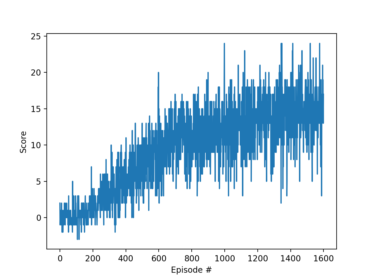
Figure 16. Repo run scores: ① random, ② a noisy climb, ③ near the solve bar.
One value per move, learned with a network, a replay buffer and a target network.
On this page
In reinforcement learning an agent tries moves, receives a score, and learns which moves lead to a higher score.
The running example is an agent that collects bananas in a Unity ML-Agents arena (ML-Agents is Unity's toolkit for game-like training worlds); the code is in the Value-based-methods repo. The agent picks one of four moves (forward, backward, turn left, turn right) and gets +1 for a yellow banana and −1 for a blue one.
A Deep Q-Network (DQN) learns one number per move, the Q-value: how much future score that move is worth in the current situation. A neural network maps what the agent senses to those numbers, the agent takes the move with the biggest one, and training pushes each number toward the reward that followed plus the value of the next situation.
DQN acts every step but learns only every fourth step (Figure 1).
The world is a square room of yellow and blue bananas. The episode score is yellows minus blues when a fixed clock runs out.
The agent senses the room as 37 numbers: its velocity plus ray sensors, each reporting the distance to the nearest yellow banana, blue banana or wall.
The arena counts as solved when the average score over 100 consecutive episodes reaches 13, the solve rule of the Udacity deep RL course project the repo comes from.
The snippet plays one episode. brain_name keys the arena's one agent in the output of env; agent holds the network and the replay buffer (Section 6); eps is the chance of a random move (Section 3).
DECAY, EPS_MIN = 0.998, 0.01

out = env.reset(train_mode=True)
info = out[brain_name]
s = info.vector_observations[0]
score = 0
while True:
    a = agent.act(s, eps)
    out = env.step(a)
    info = out[brain_name]
    r = info.rewards[0]
    obs = info.vector_observations
    s_next = obs[0]
    d = info.local_done[0]
    agent.step(s, a, r, s_next, d)
    score += r
    s = s_next
    if d:
        break
eps = max(eps * DECAY, EPS_MIN)EPS_MIN.One banana step carries the example: from situation s the agent moves forward onto a yellow banana, +1. What the agent wants is all the reward still to come, the return (Figure 3).
The same move can land in different spots, so its value is the return it earns on average (Figure 4).
The Bellman equation skips the wait for whole episodes: it peels off the first reward and lets the best next Q-value stand in for the rest (Figure 5).
The guesses at s′ are the table's, not true averages, so the target 3.475 disagrees with the stale entry for forward, 2.0. Q-learning moves the entry part of the way (Figure 6); over many visits it hovers near the true average, about 3.41.
alpha below) moves the entry only that share of δ, so one lucky step cannot overwrite everything learned. The grid in Section 4 runs these lines; Section 6.3 keeps them with a network.The snippet runs one tabular update; a is the move just taken.
best = max(Q[s_next])
target = r + gamma * best
td = target - Q[s][a]
Q[s][a] += alpha * tdtd, the TD error δ (line 2), and moves the entry a share α of it (line 3).Always taking the best-known move never tries anything new, so with chance epsilon, ε, the agent moves at random.
Epsilon starts at 1.0, all random, and shrinks after every episode (Figure 7).
Random moves still teach the agent, because Q-learning is off-policy: its target uses the best next move, whatever move comes next.
A 6 by 6 banana room is the largest table you can watch fill; the real agent's 37 numbers need the network of Section 6.
Figure 8. Q-learning on a 6 by 6 grid: squares near yellows turn orange first.
The state is the square plus which yellows are still uneaten. Toy α 0.3, γ 0.9, ε decay 0.99; the real run uses Adam (gradient descent that sizes each weight's step from its recent gradients) at 5e-4, γ 0.99, decay 0.998.
One agent keeps ε at 1.0; the other uses the rule of Section 3 with 0.97 instead of 0.998, so the race ends fast.
Figure 9. Same learning rule; only the decaying ε reaches a high score.
Toy α 0.3, γ 0.9.
Tabular Q-learning (Watkins, 1989) needs one row per situation, too many for 37 continuous numbers, so DQN (Mnih et al., 2015) replaces the table with a neural network: 37 numbers in, four Q-values out.
A network shares weights across situations, so one update shifts many Q-values; training turns unstable in two ways, and DQN adds one fix for each.
The DQN paper learned control from raw screen pixels with a convolutional network (layers that scan the input for small local patterns), stabilized by both fixes (Figure 10). The banana agent feeds 37 numbers instead of pixels.
The first fix is experience replay. Consecutive steps are almost identical, so training on them in order fits one corner of the arena and forgets the rest.
A replay buffer stores past steps, and training draws random batches from it (Figure 11).
import random
from collections import deque

BUFFER_SIZE = 100_000
BATCH = 64
buf = deque(maxlen=BUFFER_SIZE)
buf.append((s, a, r, s_next, d))
batch = random.sample(buf, BATCH)The second fix is the target network. If the network being trained also computes its own target, every gradient step (one small weight change that lowers the loss) moves the guess and the target together, and the Q-values can keep growing instead of settling.
A second copy computes the targets and trails the live network by a small share per update, the repo's soft update. The 2015 DQN paper instead copied the live network into it every 10,000 updates, frozen in between.
One step is the Section 2 update with three changes: a network replaces the table, a slow copy computes the target, and the correction becomes a gradient step on the squared TD error (Figure 13); Figure 14 follows one weight.
learn_step (Section 10) multiplies the γ term by 1 − d, where d (done) is 1 at an episode end. The arena ends every episode on a clock, so a time-out counts as a true end, a small approximation. The repo uses the Double target of Section 9, which edits only this max.The same three lines in PyTorch, with opt an Adam optimizer over q_live; s, a, r and s_next are a batch of 64 steps.
import torch
import torch.nn.functional as F

GAMMA, TAU = 0.99, 1e-3

def soft_update(tgt, src):
    old = list(tgt.parameters())
    new = list(src.parameters())
    with torch.no_grad():
        for t, p in zip(old, new):
            t.lerp_(p, TAU)

with torch.no_grad():
    q_next = q_target(s_next)
    best = q_next.max(1, True)
    y = r + GAMMA * best.values
q_sa = q_live(s).gather(1, a)
loss = F.mse_loss(q_sa, y)
opt.zero_grad()
loss.backward()
opt.step()
soft_update(q_target, q_live)soft_update: moves each target weight a fraction τ toward the live weight.max(1, True) keeps it a (64, 1) column (line 1).Step 1: Act
Figure 15. One DQN training step, in five parts.
The lines are the card of Section 6.3; the numbers follow memory 1 of Figure 13.
Epsilon (Section 3) sets the pace.
Figure 16. Repo run scores: ① random, ② a noisy climb, ③ near the solve bar.
The repo's network is a Dueling Double DQN: Double changes the target, Dueling how each Q-value is built (both on Value-Based RL).
The max of noisy guesses runs high even when no move beats another (Figure 17, left). Double DQN (van Hasselt et al., 2016) lets the live network pick and the target network score.
learn_step in Section 10 computes it. TD3 (Twin Delayed DDPG, Continuous-Action Actor-Critic, section 2) uses the same idea.Dueling (Wang et al., 2016) splits the network into a situation value and each move's edge, then adds them (Figure 18).
QNetwork below builds the sum.The repo's network as a module; q_live and q_target are the two copies used above.
import torch.nn as nn
import torch.nn.functional as F
from torch.optim import Adam

class QNetwork(nn.Module):
    def __init__(self, h=64):
        super().__init__()
        self.l1 = nn.Linear(37, h)
        self.l2 = nn.Linear(h, h)
        self.v = nn.Linear(h, 1)
        self.adv = nn.Linear(h, 4)

    def forward(self, s):
        f = F.relu(self.l1(s))
        f = self.l2(f)
        h = F.relu(self.l2(f))
        v = self.v(h)
        a = self.adv(h)
        m = a.mean(1, True)
        return v + a - m

q_live = QNetwork()
q_target = QNetwork()
w = q_live.state_dict()
q_target.load_state_dict(w)
params = q_live.parameters()
opt = Adam(params, lr=5e-4)qn.py.Figure 19 lists the repo's settings; Stable-Baselines3 has a widely used PyTorch DQN.
Acting costs one forward pass; a learning step runs both networks on a batch of 64. The 100,000-step buffer is about 30 MB as 32-bit floats.
| Setting and repo value | Raising it | Lowering it |
|---|---|---|
| Network 37 in, 64-unit layers, V (1) and A (4) | more capacity, slower | cheaper, may underfit |
| Replay buffer 100,000 | more varied, adapts slower | forgets faster, batches alike |
| Batch 64 | steadier, more compute | cheaper, noisier |
| Learn every 4 steps | fewer updates, cheaper | more reuse; can chase noise |
| Adam learning rate 5e-4 | faster; Q-values can diverge | steadier, slower |
| Discount γ 0.99 | far rewards count more | only near rewards count |
| Target update τ 1e-3 | faster, less stable; τ = 1 copies | steadier; τ = 0 freezes |
| ε start, floor 1.0, 0.01 | more random moves late | a floor of 0 stops exploring |
| ε decay × 0.998 per episode | explores longer | settles on the first route that scores |
learn_step is the repo's learning step, using q_live, q_target, opt and soft_update from above.
import torch
import torch.nn.functional as F

GAMMA, TAU = 0.99, 1e-3

@torch.no_grad()
def td_target(r, s_next, done):
    live_q = q_live(s_next)
    a2 = live_q.argmax(1, True)
    tgt_q = q_target(s_next)
    q_t = tgt_q.gather(1, a2)
    keep = 1 - done
    return r + GAMMA * q_t * keep

def learn_step(batch):
    s, a, r, s_next, done = batch
    y = td_target(r, s_next, done)
    q_sa = q_live(s).gather(1, a)
    loss = F.mse_loss(q_sa, y)
    opt.zero_grad()
    loss.backward()
    opt.step()
soft_update(q_target, q_live)keep is 0 at the end of an episode.Three details keep this loop correct.
done; without it the last step of an episode takes value from the next episode.done as a float; PyTorch cannot subtract a bool tensor from 1.a, r and done as (64, 1) columns; a (64,) reward broadcast against (64, 1) values becomes (64, 64), and the loss only warns.Figure 20. The trained agent holds course and curves around blue bananas.
DQN takes the max over four Q-values; a continuous action, such as a Reacher arm's joint torque, any real number from −1 to 1, leaves no list to take the max over.
Deep Deterministic Policy Gradient (DDPG): Actor and Critic solves this by keeping the Q-value and adding a second network, the actor, that outputs the action directly.