← All tutorials

On this page

Gated RNNs: GRU and LSTM

A gate is a small layer ending in a sigmoid (from Logistic Regression), so its output, between 0 and 1, scales how much old memory survives and how much new input enters. With a gate near keep, memory and gradient pass through a step unchanged, which the plain RNN cannot do.

This page builds on RNN Basics: Recurrence and Backpropagation Through Time, which teaches the plain recurrent cell and why its gradients vanish.

The plain cell runs the same two lines at every step:

Backpropagating through many such steps multiplies the gradient by one factor per step, so it fades over a few dozen steps (Why gradients vanish or explode, in RNN Basics: Recurrence and Backpropagation Through Time).

1 Gated Recurrent Unit (GRU)

The GRU introduces gates to control what information to keep and what to forget.

Take "Ramin wrote the best tutorial, he did it again!". A vanilla RNN might overwrite "Ramin" and forget who "he" was; a GRU's update gate can say "don't overwrite Ramin, hold on to that memory." A language model meets this all the time: to predict the next words it must link "he" back to a name many tokens earlier.

When the update gate keeps the old memory, the hidden state is copied straight to the next step: no multiplication, no tanh, an identity connection. Gradients flow back along that same path unchanged, which is how the GRU beats vanishing gradients.

1.1 Gates decide what to keep and what to forget

There are 2 gates, both little feedforward networks with a sigmoid activation, so their outputs are between 0 and 1.

• The update gate asks "Keep the old hidden state or update it?" 0 means keep the old memory, 1 means overwrite it with new memory.
• The reset gate asks "When computing new candidate memory, how much of the old memory should I ignore?"
• The candidate hidden state is a proposal for new memory. With the reset gate at zero, the candidate ignores past memory and depends only on the input.

The update is a weighted average of the old memory and the candidate, and the network learns the gate setting from data, per step, per neuron. Figure 1 draws this as dataflow.

1.2 One GRU step, in code

The whole cell is the five card lines above, as one function: each nn.Linear holds one W and its bias, torch.cat builds the stacked vector, and the names match the cards:

import torch
from torch import nn

# input and hidden sizes
d_in, d_h = 8, 16
d = d_in + d_h
W_z = nn.Linear(d, d_h)
W_r = nn.Linear(d, d_h)
W_h = nn.Linear(d, d_h)

def gru_step(x_t, h):
    # h is h_t-1: (batch, d_h)
    xh = torch.cat([x_t, h], -1)
    z = W_z(xh).sigmoid()
    r = W_r(xh).sigmoid()
    m = r * h
    xm = torch.cat([x_t, m], -1)
    h_tilde = W_h(xm).tanh()
    keep = (1 - z) * h
    return keep + z * h_tilde

1. 1Builds one weight matrix with its bias for each of W_z, W_r and W_h, each reading the stacked vector.
2. 2Stacks input and memory and computes the two gates, the first card.
3. 3Filters the memory, builds the candidate and blends: keep is the old memory times the keep share (1 − z), the second card.

The GRU has no separate cell state (a memory stream beside the hidden state); the update gate's identity path is enough to preserve long-term memory.

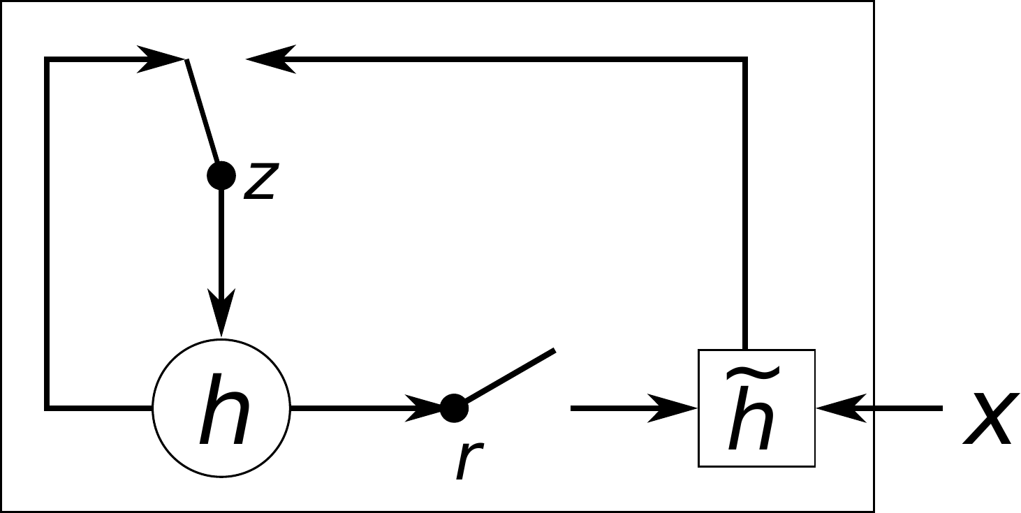
This is the paper that introduced the GRU (Cho et al., EMNLP 2014). Figure 2 is the paper's Figure 2, its real hidden-unit diagram, with an excerpt of its original caption.

That paper and PyTorch put z on the old state; this page follows Chung et al. (2014), which puts z on the candidate. PyTorch's nn.GRU also applies the reset after the matrix rather than before it; the same paper found the two forms perform alike.

2 Long Short-Term Memory (LSTM)

LSTM (Long Short-Term Memory) separates memory into two parts and uses three gates to carefully control what flows into, out of, and stays within these memories.

The cell state C is the memory tank: it runs through the cell with no squashing nonlinearity, so information and gradients ride it across hundreds of steps. The hidden state h is the short-term read, filtered from the tank for this step.

Three gates guard the tank, and each one is a question the network asks every step:

1. The forget gate asks "Do I still need this?" It looks at the old level and drains what stopped mattering.
2. The input gate asks "Is this worth writing down?" It decides how much of the new candidate actually gets poured into the tank.
3. The output gate asks "What do I show right now?" It filters the tank's level down into the hidden state.

2.1 The LSTM update

The forget gate scales yesterday's level, the input gate scales today's pour (the candidate), and they add. The cell state is only ever scaled and added, never squashed, which is why gradients walk straight back down the highway. The output gate then picks how much of the squashed level to show as h. Each gate is a sigmoid of the input and the previous hidden state. Figure 5 draws this as dataflow.

Take an always-listening device: once it hears the wake word, the cell must hold "wake word heard" across many quiet audio frames until the command arrives.

Why does the gradient survive on the cell line? Why gradients vanish or explode (in RNN Basics: Recurrence and Backpropagation Through Time) showed that every step back multiplies the gradient by one factor. Put the plain RNN's factor next to the gated ones:

Back on the always-listening device, the cell should keep the wake word, not the louder door slam that comes three steps later. Here the forget gate stays open, and the pour sizes are illustrative.

2.2 The forget gate was added later

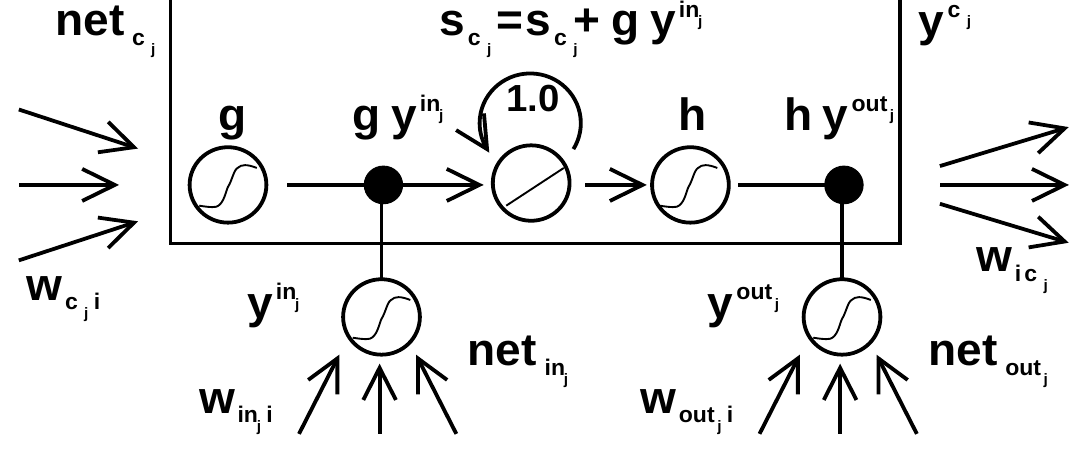
This is the paper that started all of this (Hochreiter and Schmidhuber, 1997): a memory cell with a self-loop of weight exactly 1.0, so the error can cycle forever without shrinking, plus gates that open and close access to it. Figure 8 is the paper's Figure 1, its real memory-cell architecture, with an excerpt of its original caption.

There is no forget gate in this figure. The 1997 LSTM had only input and output gates; the forget gate arrived three years later, from Gers et al. ("Learning to Forget," 2000). The LSTM on this page is the post-2000 version.

3 Long sequences expose the vanilla RNN

How long does each cell hold one event? Figure 9 feeds the same single spike to a plain RNN, a GRU and an LSTM. The cost line under each lane counts the weights of one scalar cell of that kind, three per block (input weight, memory weight, bias): one block for the plain RNN, three for the GRU (update gate, reset gate, candidate) and four for the LSTM (three gates and the candidate). Each weight costs about one multiply and one add per step, and 1×, 3× and 4× give the cost per step next to the plain RNN's.

In the field, bidirectional LSTMs, one reading forward and one backward, transcribe speech when trained with the CTC loss.

In practice you never write these cells by hand. PyTorch has them built in:

from torch import nn
# x: (batch, seq, feat)
lstm = nn.LSTM(
    input_size=28,
    hidden_size=128,
    num_layers=2,
    batch_first=True)
# output: every step, last layer
# hn, cn: final states per layer
output, (hn, cn) = lstm(x)
# GRU: same, no cell state
# output, hn = gru(x)

1. 1Builds a two-layer LSTM for inputs of 28 features with 128 hidden units.
2. 2Runs the sequence and returns every step of the last layer plus the final hidden state hn and cell state cn of each layer.
3. 3The GRU call is the same with no cell state.

GRUs typically achieve similar results to LSTMs with fewer parameters: no separate cell state, two gates instead of three. If you are not sure which to pick, start with a GRU.

4 Training problems and fixes

• Don't draw a fresh dropout mask at every timestep inside the recurrence. Dropout (in Regularization and Data Augmentation) randomly zeroes activations during training, and a new mask at every step keeps cutting the memory the cell carries forward. Apply it between stacked layers, as the dropout argument of PyTorch's nn.LSTM and nn.GRU does, or share one mask across all timesteps, which is variational dropout (Gal and Ghahramani, 2016).
• Detaching only h breaks truncated BPTT for an LSTM. The cell state C still links back to the previous chunk, whose graph that chunk's loss.backward() already freed, so the next backward raises PyTorch's "Trying to backward through the graph a second time" error. Detach the whole (h, c) state between chunks. retain_graph=True does not help: the loop in RNN Basics: Recurrence and Backpropagation Through Time steps the optimizer after each chunk, so the next backward fails with an in-place modification error, and without those steps the graph, memory and time grow.

When do RNNs still make sense? Transformers won the long-sequence game because attention sees everything at once. RNNs are still the right call for streaming data where you must decide now with constant memory: real-time sensor streams, on-device keyword spotting, low-latency control.

Gating fixed the memory problem, but RNNs still read one step at a time, which makes training slow on long sequences. The next idea drops recurrence entirely: let every position look directly at every other position. That is Transformers.

5 References

1. Cho et al. (2014). Learning Phrase Representations using RNN Encoder-Decoder for Statistical Machine Translation. EMNLP. arXiv:1406.1078.
2. Hochreiter & Schmidhuber (1997). Long Short-Term Memory. Neural Computation 9(8).
3. Gers et al. (2000). Learning to Forget: Continual Prediction with LSTM. Neural Computation 12(10).
4. Chung, Gulcehre, Cho, Bengio (2014). Empirical Evaluation of Gated Recurrent Neural Networks on Sequence Modeling. arXiv:1412.3555.
5. Gal & Ghahramani (2016). A Theoretically Grounded Application of Dropout in Recurrent Neural Networks. NeurIPS. arXiv:1512.05287.