Principal component analysis (PCA) finds the directions along which data varies most and keeps only those. The running example is the Olivetti faces, 400 photos of 40 people at 64 by 64 pixels; PCA rebuilds each from about 10 weights on face-shaped directions called eigenfaces.
Figure 1. Each box's marker is the number of the section that teaches it.
PCA runs once, before anything uses it, in one pass over all the faces. It keeps the mean face and the top directions; encoding a new face is one dot product per direction.
1 Why a few directions are enough
Every face is a point in 4,096-dimensional space, one coordinate per pixel.
Figure 2. The corners 1 never change, so coding them adds nothing; faces differ at 2.
Neighboring pixels brighten and darken together, so one direction can describe many pixels at once, and a 10-number code only needs the regions that vary between faces.
2 Principal component analysis
Faces all have eyes above a nose above a mouth, so the cloud is stretched along some directions and flat along others.
The directions of biggest stretch are the principal components, each at a right angle to the ones before. Keeping the top k turns each face into k numbers. Curved clouds need nonlinear maps such as t-SNE.
Figure 3. Faces vary most along 1 and less along 2; PCA keeps the long directions and drops the flat ones.
Each direction is a vector of 4,096 numbers, so it reshapes into a 64 by 64 image, bright where faces differ one way along it and dark where they differ the other way. The Eigenfaces paper (Turk and Pentland, 1991) named it: "a sort of ghostly face which we call an eigenface."
3 The PCA algorithm
Five steps turn 4,096 pixels into a 10-number code. The pca notebook in the Machine-Learning-Concepts repo runs them from scratch in numpy.
3.1 Center the data
Subtract the mean face, the pixel-by-pixel average of all 400 faces, from every face. Each face has 4,096 pixels, so the covariance built next is 4,096 by 4,096, made from only 400 centered faces; its rank, the number of independent directions it holds, is at most 399. Step 1 of Figure 5 draws the mean face and step 2 a centered face.
PCA first subtracts the average face so every pixel measures a difference from it.
μ = 1nΣx
The mean face μ is every face x added up (Σ) and divided by the count n. Variance is measured around the mean, so without centering the first component would point at the average face instead of along the variation.
Xc = X − μ
Xc is each face minus the mean, so only what makes each face different remains: brighter-than-average pixels go positive, darker ones negative.
So centered data has its average at the origin, and what is left is how faces differ. The eq card in Section 3.2 measures how pixels vary together.
3.2 The covariance matrix
The covariance matrix records how pixels vary together; its diagonal holds each pixel's own variance.
The covariance matrix records how every pair of pixels rises and falls together.
C = 1nXcTXc
It is built from the centered faces of the eq card in Section 3.1. C averages the centered faces times their transpose (T flips rows and columns). Each entry is positive when two pixels move together and negative when they move opposite. Probability pages write a covariance as Σ; here Σ is the sum sign and C the covariance.
An eigenvector is a direction in pixel space; its eigenvalue is a single number, how much the data varies along that direction.
Figure 4. Multiplying by C only stretches the eigenvector v1; any other direction u2 also turns.
Sort them by eigenvalue, biggest first, and reshape the first eigenvector into a 64 by 64 image: that is the first eigenface.
RecapWhat does an eigenvector’s λ say about the faces? Home: eigenvectors
The principal components are the directions the covariance matrix only stretches.
var(u) = uTCu
C is the covariance of the eq card in Section 3.2. The variance of the centered faces along a unit-length direction u. It is largest when u is the top eigenvector v, and there it equals that eigenvector's eigenvalue λ; the next eigenvector wins among directions at right angles to the first. That is why the eigenvectors are the principal components.
Cv = λv
Multiplying the covariance by an eigenface v just stretches it, by its eigenvalue λ, without rotating it. v is a direction of variation and λ is how much variation that direction holds: big eigenvalue, faces differ a lot along it; small eigenvalue, nearly constant, safe to drop.
Dot a centered face with each eigenface; the result is large when the face contains much of that eigenface. 4,096 numbers in, k numbers out. The tools on this page shrink the faces to 32 by 32: step 5 of Figure 5 draws one face’s code at k = 8 as eight bars, and the face tool of Section 5 rests at a 10-number code.
Encoding keeps a face’s coordinates on the top k directions.
z = XcVk
Vk holds the top k eigenvectors of the eq card in Section 3.3, one per column. The code z that encodes this face is the centered face dotted with each of the top k eigenfaces Vk, each dot measuring how much of that eigenface this face has, its mix of eigenfaces. Those k numbers are the compressed code for the face.
So the code is the face in the top directions, k numbers in place of 4,096 pixels; the eq card in Section 3.5 rebuilds it.
3.5 Reconstruct (decode)
Start from the mean face and add back each eigenface, scaled by how much of it this face had. From its 8 code numbers, the last step of Figure 5 gives a blurred but recognizable copy; at k = 0 only the mean face is left.
Decoding adds the mean face back to the code times the directions.
x̂ = μ + zVkT
z is the code of the eq card in Section 3.4 and μ the mean face of the eq card in Section 3.1. The rebuilt face x̂ starts from the mean face μ and adds back each eigenface scaled by its code amount in z, which is z times Vk with the raised T, the transpose, the top k eigenfaces with their rows and columns flipped. With k small you get a blurred average of the right person; with k bigger the details fill in.
So encode then decode is PCA’s compression; the card under Figure 5 runs the steps in one pass.
So a face is the mean plus a weighted sum of eigenfaces: the eigenfaces form a new basis, as sine waves do in Fourier analysis.
Figure 5. A face is the mean face plus weights on eigenfaces; adding them back rebuilds it.
One face goes in, an 8-number code comes out, and the code rebuilds the face: subtract the mean, find the directions of biggest variation, write the face as a short code, and rebuild from the code.
μ = 1nΣx
Each line reads as in its own card, from the eq card in Section 3.1 on. The average face is the sum of every face divided by the count.
Xc = X − μ
Subtract the average from every face, so only what makes each face different remains.
C = 1nXcTXc
The covariance multiplies the centered faces by their transpose to show which pixels vary together.
Cv = λv
The eigenfaces are the directions v that the covariance C only stretches, by the amount λ. λ is the variation of the faces along v, so sorting by λ ranks the eigenfaces from most to least informative.
z = XcVk
Projecting the face onto the top k eigenfaces gives its code, a short list of mix amounts.
x̂ = μ + zVkT
The rebuild mixes the top eigenfaces by the code amounts and adds the average face back.
X the facesμ the mean faceXc each face minus the meanC the covariance, which pixels vary togetherv an eigenface, a direction of variationλ how much variation that direction holdsz the code, this face's mix of eigenfacesx̂ the rebuildn the face count; Σ add upVk the top k eigenfacesT the transpose, which flips rows and columns
The six steps in NumPy, with X holding one face per row (400 by 4096).
import numpy as np
K = 10  # the face tool's rest; Figure 5 uses 8
mu = X.mean(axis=0)
Xc = X - mu  # (400, 4096)
C = Xc.T @ Xc / len(X)
lam, V = np.linalg.eigh(C)
order = np.argsort(lam)[::-1]
lam, V = lam[order], V[:, order]
V_k = V[:, :K]  # eigenfaces
z = Xc @ V_k  # (400, K)
X_hat = mu + z @ V_k.T
3Eigenvectors sorted by eigenvalue; the top K are eigenfaces, step 3.3.
4Encode every face to K numbers, step 3.4.
5Decode back to pixels, step 3.5.
4 PCA in scikit-learn
scikit-learn fits the same model.
from sklearn.datasets import fetch_olivetti_faces
from sklearn.decomposition import PCA
faces = fetch_olivetti_faces()
X = faces.data  # (400, 4096)
pca = PCA(n_components=10)
z = pca.fit_transform(X)  # 400x10
1Loads the 400 faces as rows.
2Learns 10 eigenfaces and returns each face's 10-number code.
5 Reconstruction from k components
The tool rebuilds faces shrunk to 32 by 32 pixels. From their eigenvalues, the first eigenface keeps 25.39% of the variance, 7 keep 63.38% (the rest of Figure 8), 10 keep 69.22% (the tool’s rest) and 50 keep 90.49%.
The variance kept by k directions is the sum of their eigenvalues over the total.
kept(k) = Σkj=1λjΣjλj
The eigenvalues are those of the eq card in Section 3.3. Each eigenvalue λj is the variation along eigenface j. The top adds the first k; the bottom adds all of them, the dataset's total variation. The eigenvalues are sorted largest first, so kept(k) climbs fast and then flattens; it reaches 1 once k equals the data's rank, here at most 399 for 400 centered faces. Raise k and the rebuild sharpens toward the original; lower it and faces blur toward the mean face, which is all that is left at k = 0. scikit-learn keeps every component by default (n_components=None).
So k is chosen from this curve: it climbs fast for the first few eigenfaces and then flattens. The eq card in Section 7 rescales the code.
k = 10
Figure 6. By k = 10 the face is recognizable; each eigenface past 10 helps less.
eigenfaces used in this rebuild (first k)remaining eigenfaces (not used)
6 Recognizing faces with eigenfaces
To recognize a face, project it onto the eigenfaces and name the known person whose weights are nearest; a face far from everyone is unknown, and an image whose rebuild from the eigenfaces is far from the image itself is not a face.
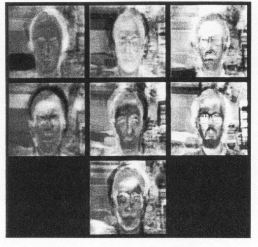
Figure 7. "Seven of the eigenfaces calculated from the input images of [the paper's] Figure 1," as the Eigenfaces paper captions its Figure 2.
One eigenface per numbered cell, biggest variance first; bright and dark are the two opposite ways along it. From the Eigenfaces paper (J. Cognitive Neuroscience 1991). doi:10.1162/jocn.1991.3.1.71
Variance share per eigenface, Olivetti faces at 32 by 32
Figure 8. Eigenface 1 explains 25.39% of the variance and eigenface 7 only 2.49%.
7 PCA variants
Whitening (whiten=True, off by default) divides each code by its spread so every direction has unit variance; the first eigenfaces stop dominating, but noisy low-variance directions get boosted too. Whitening is also the first step of Independent Component Analysis (ICA), which separates mixed recordings into their sources.
Whitening divides each code by its spread so every direction has variance 1.
z̃j = zj√λj
It rescales the code of the eq card in Section 3.4 using the eigenvalues of the eq card in Section 3.3. zj is a face's code along eigenface j, λj is that eigenface's eigenvalue, and z̃j is the whitened code: dividing by the square root of the eigenvalue leaves every direction with variance 1 when λ uses the 1n − 1 convention, as scikit-learn does; with the 1n covariance of the eq card in Section 3.2 it is nn − 1, about 1.
So whitened codes weigh every kept direction equally; for 400 faces the two conventions differ by only a quarter of a percent. End of the chain.
Kernel PCA runs PCA after a kernel lift, as on the SVM page, for curved data; randomized SVD (singular value decomposition) sketches a huge matrix with random projections first; robust PCA down-weights a few wild samples.
from sklearn.datasets import fetch_olivetti_faces
from sklearn.decomposition import PCA
from sklearn.model_selection import train_test_split
from sklearn.neighbors import KNeighborsClassifier
from sklearn.pipeline import make_pipeline

faces = fetch_olivetti_faces()
X, y = faces.data, faces.target
split = train_test_split
parts = split(X, y, stratify=y)
Xtr, Xte, ytr, yte = parts
pca = PCA(50, whiten=True)
knn = KNeighborsClassifier(1)
model = make_pipeline(pca, knn)
model.fit(Xtr, ytr)
acc = model.score(Xte, yte)
1Holds out a stratified test split of faces.
2Whitened PCA codes (Section 7) feed a 1-nearest-neighbor classifier.
3Fits on training faces only, then test accuracy.
Setting
Where it enters
Raise it
Lower it
Default
n_components, k
Eigenfaces kept in the share card
Sharper rebuild, longer code
Blurrier, toward the mean face
None, keep all; a float in (0, 1) keeps that share of variance
whiten
Divides each code by its spread
Turned on, every direction counts equally; turned off, the top eigenfaces dominate
False
svd_solver
How the directions are computed
"randomized" sketches big data; "full" is exact
"auto", chosen by data size
PCA centers but does not scale the data and fits once by SVD of the centered data, which gives the same eigenfaces without building C. Encoding afterwards is one matrix product, cheap enough for every request.
Fit PCA on the training split only, or test faces leak into the directions, and standardize features measured in different units first.
Cause
Symptom
Fix
Features on different scales
the biggest-scale feature takes the first components
standardize each feature to spread 1 first
A few outliers
one wild sample tilts a direction toward itself
remove them or use robust PCA
Curved data
straight directions miss the shape, so k must grow large
Turk, M., et al. (1991). Eigenfaces for Recognition. Journal of Cognitive Neuroscience. doi:10.1162/jocn.1991.3.1.71
Samaria, F., et al. (1994). Parameterisation of a Stochastic Model for Human Face Identification. Proceedings of the 2nd IEEE Workshop on Applications of Computer Vision.