 1234
 12
 34
On this page
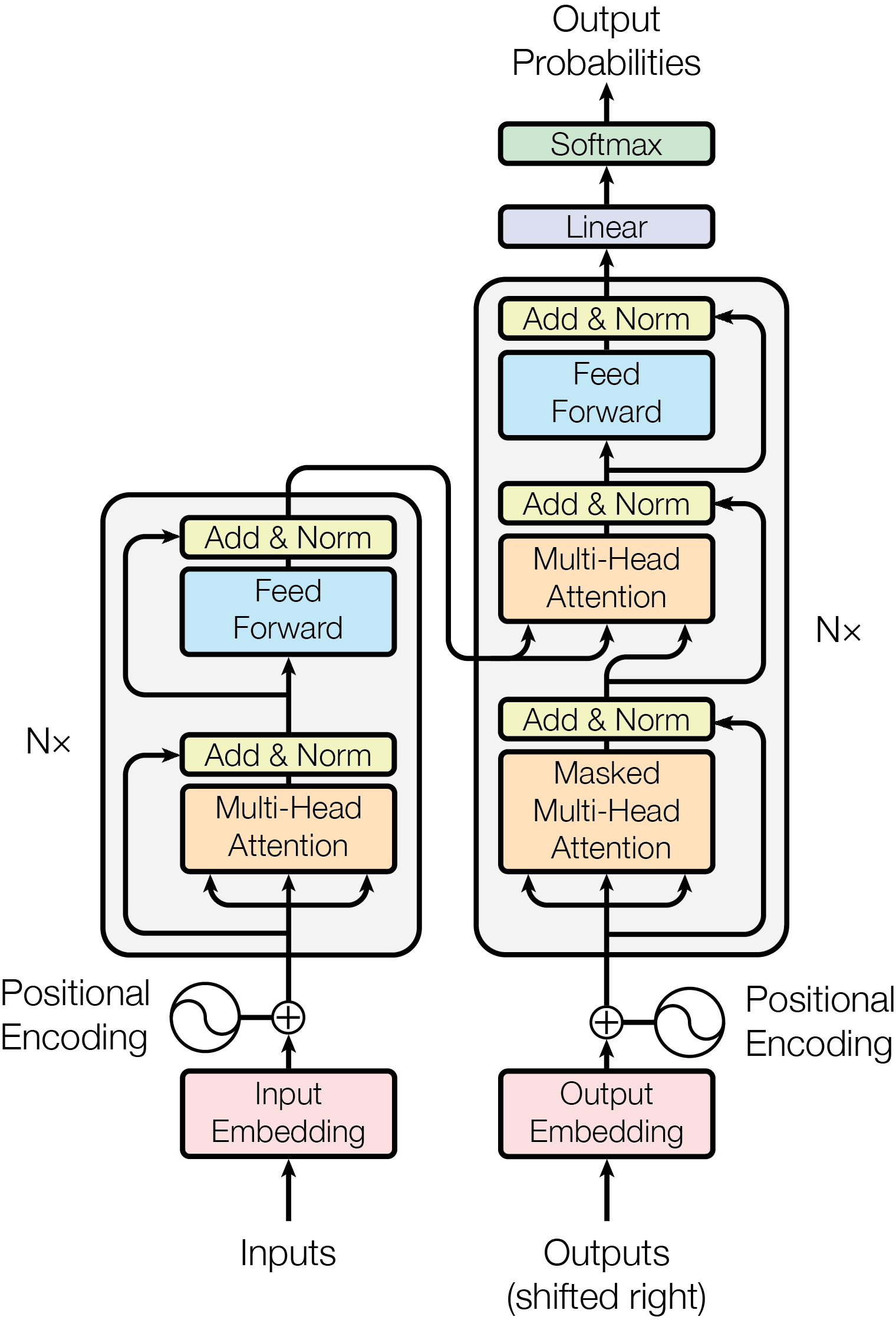
A Transformer is a stack of identical blocks, all trained together so the top vectors predict well. Each block mixes information across tokens with attention, then updates every token on its own with a small feed-forward network. Every block runs on every forward pass over all tokens, in training and in generation.
As in Attention, each token (a word or word piece) is a vector of dmodel numbers making a query, a key and a value, stacked as rows of Q, K and V (key length dk). Several heads run attention side by side, and in a decoder a causal mask stops each token from seeing later ones.
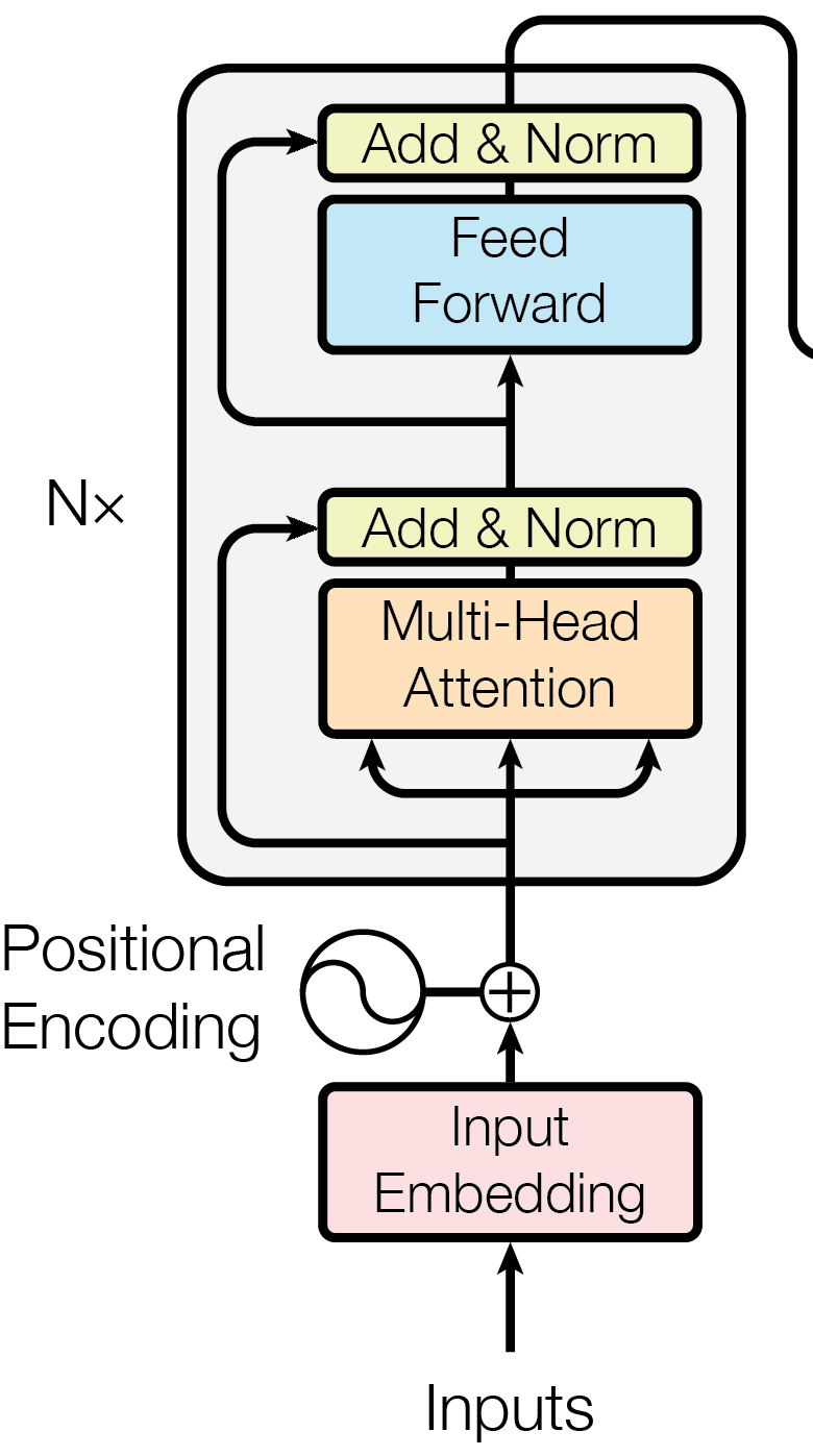
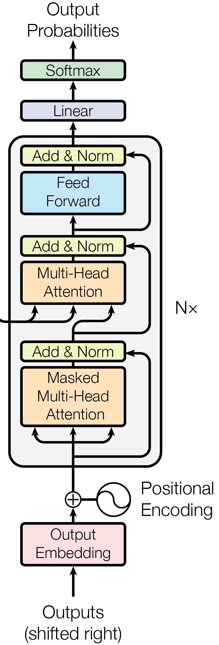
A block runs two sublayers in turn: attention mixes information between tokens, then a small feed-forward network (FFN), two linear layers with a ReLU nonlinearity (it zeroes negative numbers) between them, transforms each token on its own. Each sublayer adds its result back onto the token's vector instead of replacing it, so that running vector, the residual stream, flows straight up through every block.
LayerNorm (LN; Ba et al., 2016) rescales a token's vector to mean 0 and variance 1 using only that token's numbers (Section 2 has the details). With LN before each sublayer, a layout called Pre-LN, one block is two lines plus one final LayerNorm:
The Pre-LN block in PyTorch; shape (B, T, d) goes in and comes out.
import torch
import torch.nn as nn
from torch.nn import MultiheadAttention as MHA

class Block(nn.Module):
    def __init__(self, d, h, d_ff):
        super().__init__()
        self.ln1 = nn.LayerNorm(d)
        self.ln2 = nn.LayerNorm(d)
        self.attn = MHA(d, h, batch_first=True)
        self.W1 = nn.Linear(d, d_ff)
        self.W2 = nn.Linear(d_ff, d)

    def forward(self, x, mask=None):  # x (B, T, d)
        y = self.ln1(x)
        out, _ = self.attn(y, y, y, attn_mask=mask)
        x = x + out                      # x + Attn(LN(x))
        u = self.W1(self.ln2(x)).relu()  # (B, T, d_ff)
return x + self.W2(u) # x + FFN(LN(x))Passing one normalized tensor as query, key and value makes this self-attention.
LayerNorm normalizes each token using only that token's own numbers:
BatchNorm (Ioffe and Szegedy, 2015), the usual choice in image models, instead averages each feature over every token of every sequence in the batch:
Both kinds of mean on one batch, then LayerNorm on a single token.
import torch
import torch.nn.functional as F

B, T, d = 32, 10, 512
x = torch.randn(B, T, d)
ln_mean = x.mean(dim=-1)      # LayerNorm, (B, T)
bn_mean = x.mean(dim=(0, 1))  # BatchNorm, (d,)

one_token = torch.tensor([1.0, 2.0, 3.0])
print(F.layer_norm(one_token, (3,))) # [-1.22, 0., 1.22]BatchNorm's batch averages mix in other sentences and padding, and at inference it switches to stored averages; LayerNorm uses one token's own numbers, so training and inference match.
Warmup means starting with a tiny learning rate and ramping it up over the first few thousand steps. LayerNorm can sit before each sublayer or after each add, and that choice decides whether training needs warmup. The 2017 paper put it after the add, on the stream itself, a layout called Post-LN:
Xiong et al. (2020) showed that going backward, a LayerNorm divides the gradient by the same spread it divided its input by going forward (the square root in the LN card of Section 2). So a larger input lets a smaller gradient through. In Pre-LN every block adds onto the stream and nothing rescales it, so the stream's size, the root mean square (RMS) of its numbers, grows with each block, and the final LayerNorm divides the gradient by that growing size. In Post-LN the stream is renormalized inside every block, so the last LayerNorm always divides by about the same size, and the gradient near the output stays large however many blocks are stacked. Because each LayerNorm also breaks the identity path (the Post-LN card above), that large gradient is not carried down unchanged: it is largest near the output and smaller toward the input.
Large gradients near the output mean a full-size learning rate makes the first updates there too big, and training can diverge; warmup keeps the early steps small until the gradients settle. Pre-LN's top gradient is smaller and shrinks as the stack deepens, so it can start at the full learning rate with no warmup.
Post-LN's toy gradient is 2.6× bigger.
Figure 4. 1 Pre-LN's stream grows. 2 Its gradient falls. 3 Not Post-LN's.
The original Post-LN Transformer warmed up with this schedule, then decayed.
The schedule in Python.
WARMUP = 4000

def lrate(step, d_model=512, warmup=WARMUP):
    step = max(step, 1)        # avoid 0 ** -0.5
    a = step ** -0.5           # decay term
    b = step * warmup ** -1.5  # warmup term
    return d_model ** -0.5 * min(a, b)

print(lrate(4000), lrate(16000)) # about 7e-4, then halfFigure 5. The rate peaks at step 4000; by step 12000 it is down to about 0.58 of the peak.
The paper behind that backward rule also trained Pre-LN models with no warmup and, in its words, reached "comparable results with baselines while requiring significantly less training time". One of its tests was BERT, a Post-LN stack of 12 blocks in BERT-base and 24 in BERT-large. Post-LN BERT-base was trained with 10,000 warmup steps to a peak of 1e-4; a peak of 3e-4 diverged. Pre-LN BERT-base started at 3e-4 with no warmup.
The same block builds three kinds of model, differing in the self-attention mask and whether a second stream comes in.
The 2017 translator is an encoder-decoder: the encoder reads the source sentence, and the decoder writes the translation while reading the encoder through cross-attention.
1234
12
34
The paper trained on WMT 2014 English to German and English to French on 8 NVIDIA P100 GPUs and scored translations with BLEU, which counts word sequences shared with human translations (higher is better), against ensembles (several models combined) of ConvS2S, a convolutional translation model.
Most models in use today, GPT among them, are decoder-only: one sequence, no encoder. The model predicts the next token, appends it and predicts again (autoregressive generation).
Training minimizes the cross entropy averaged over positions:
MiniGPT wraps the Block class from Section 1 with a token table, a position table and a final LayerNorm, and reuses the token table as the output layer, giving logits, one raw score per vocabulary word.
import torch
import torch.nn as nn

MAX_LEN, N_HEADS = 128, 8

class MiniGPT(nn.Module):
    def __init__(self, V, d, N):  # vocab, width, blocks
        super().__init__()
        self.tok = nn.Embedding(V, d)
        self.pos = nn.Embedding(MAX_LEN, d)
        blocks = [Block(d, N_HEADS, 4*d) for _ in range(N)]
        self.body = nn.ModuleList(blocks)
        self.ln = nn.LayerNorm(d)  # final LayerNorm

    def forward(self, idx):  # idx (B, T) token ids
        T = idx.size(1)
        x = self.tok(idx) + self.pos.weight[:T]
        mask = torch.ones(T, T, dtype=torch.bool).triu(1)
        for block in self.body:
            x = block(x, mask)
return self.ln(x) @ self.tok.weight.T # (B, T, V)Weight tying makes the output layer reuse the embedding table (both are vocabulary size by model width), saving a large block of weights.
Training MiniGPT on random toy batches, grading each position against the next token.
import torch
import torch.nn.functional as F

VOCAB, d, N, LR = 10_000, 256, 4, 3e-4
model = MiniGPT(VOCAB, d, N)
opt = torch.optim.AdamW(model.parameters(), lr=LR)
batches = [torch.randint(VOCAB, (8, 64)) for _ in range(10)]

for ids in batches:  # ids (B, T)
    logits = model(ids)
    pred = logits[:, :-1].flatten(0, 1)
    target = ids[:, 1:].flatten()  # one step later
    loss = F.cross_entropy(pred, target, reduction="mean")
    opt.zero_grad()
    loss.backward()
opt.step()At generation a setting called temperature divides the last position's logits before the softmax:
In generation, a prompt goes in and comes back with n_new tokens added.
import torch

@torch.no_grad()
def generate(model, ids, n_new, tau=1.0, max_len=128):
    for _ in range(n_new):
        z = model(ids[:, -max_len:])[:, -1]  # (B, V)
        p = (z / tau).softmax(dim=-1)
        nxt = p.multinomial(1)  # one token per row
        ids = torch.cat([ids, nxt], dim=1)
return idsmultinomial draws a token by those probabilities; Softmax, Temperature and Decoding shows top-k and top-p, which sample from only the likeliest words. Each step recomputes every earlier token's keys and values; Transformer Cost and Efficiency shows how a cache removes that.
the cat sat on the …
Figure 10. Temperature sharpens or flattens the same distribution; the order of the words never changes.
The base model's six-block encoder from PyTorch's layer, Pre-LN; shape (B, T, 512) goes in and comes out.
import torch
import torch.nn as nn

D_MODEL, HEADS, D_FF, N_LAYERS = 512, 8, 2048, 6
cfg = dict(dropout=0.1, batch_first=True, norm_first=True)
layer = nn.TransformerEncoderLayer(D_MODEL, HEADS, D_FF, **cfg)
final_norm = nn.LayerNorm(D_MODEL)
encoder = nn.TransformerEncoder(layer, N_LAYERS, norm=final_norm)

x = torch.randn(2, 10, D_MODEL)  # (B, T, d_model)
print(encoder(x).shape)  # torch.Size([2, 10, 512])
print(sum(p.numel() for p in encoder.parameters()))
# 18915328, about 12 * 512 ** 2 per block| Block | Each of the N blocks, every forward pass, every token. |
|---|---|
| LayerNorm | Per token before each sublayer (Pre-LN), every forward pass; a learned gain and bias of size d. |
| Warmup | Sets the learning rate at every optimizer step from the step count; 4000 warmup steps in the base model. More steps start slower and safer, fewer risk Post-LN diverging, and Pre-LN can skip it. |
| Next-token loss | Every training step, all T positions of a sequence graded in one pass. |
| Sampling, τ | At generation, once per new token. Temperature τ divides the logits: higher flattens toward random picks, lower sharpens toward the top token; near 0 it is greedy, always the top token, and very large it is uniform. Default 1.0, the plain softmax (temperature in Hugging Face's generation config). |
| dmodel | Width of the x every block reads and writes. Wider holds more per token at quadratic cost; narrower is cheaper and holds less. The base Transformer uses 512, with 8 heads, FFN width 2048, 6 blocks and ReLU. PyTorch's defaults match the base model, including Post-LN (norm_first=False); this page's code sets norm_first=True for Pre-LN. |
| dff | Width of the FFN's hidden vector u; 2048, four times dmodel, in the base model. Wider stores more per token, with FFN weights growing linearly as 2dmodeldff; narrower is cheaper and stores less; near 0 only attention is left. dim_feedforward in PyTorch, default 2048. |
| Blocks N | How many blocks are stacked; 6 in the base model's encoder and decoder. More blocks give each token more rounds of mixing and transforming, at cost linear in N; fewer is cheaper and shallower; at 0 only the embeddings and output layer remain. num_layers in nn.TransformerEncoder, no default. |
| Dropout | Zeroes that fraction of each sublayer's output in training, before it joins x; off at inference. More fights overfitting and slows learning, less fits faster; 0 is none, near 1 passes nothing. The base Transformer uses 0.1, also PyTorch's default. |
| Code | nn., nn.TransformerEncoder (PyTorch docs). |
norm_first=True, pass the final LayerNorm through norm=.batch_first defaults to False here too.mask passed in.What changes when one stream reads another, such as a translation reading its source? Cross-Attention.