Swipe sideways to read the labels; tap to open full size.
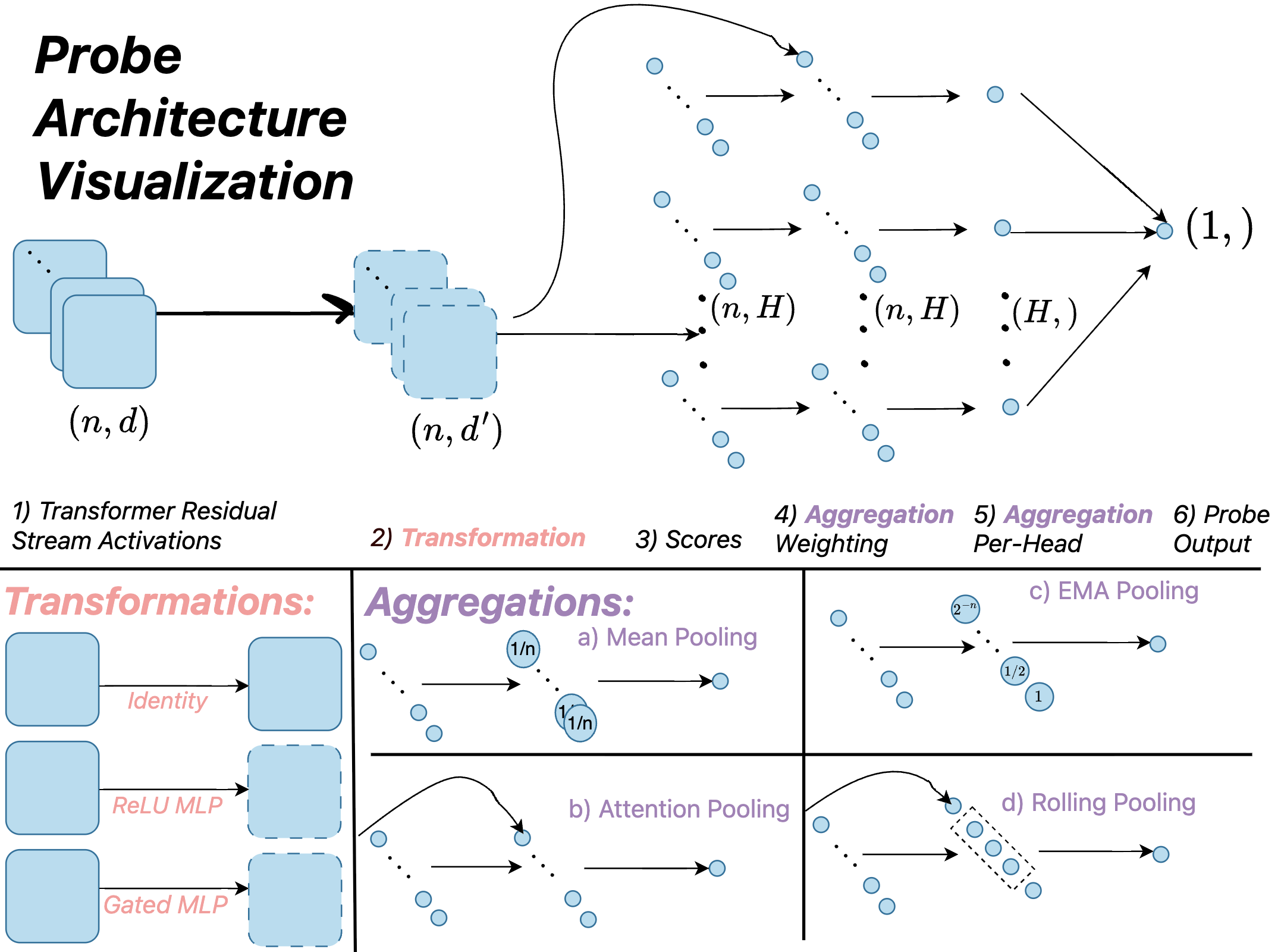
Figure 11. The paper's Figure 2: "All our probing classifiers can be composed into six states … as illustrated."
Tiny classifiers that read a model's internal activations, the lists of numbers inside the model that describe what it has understood so far, to flag harmful prompts, before it answers.
On this page
A large language model's core skill is following the instructions in your prompt, and that is also what makes it dangerous: it cannot tell which instructions deserve to be followed.
A jailbreak hides malicious instructions inside an innocent-looking prompt, and the assistant does exactly what it was told (Figure 1).
Refusal training (see Aligning Language Models with RL) does not hold against determined attackers (Nasr et al., 2025), so Kramár et al. (2026) watch prompts at deployment time instead. Google DeepMind made these probes production-ready, and their findings informed the misuse-mitigation probes in user-facing Gemini.
The obvious monitor is a second large language model, an LLM judge, asked whether each prompt is an attack; it works, but every request now costs two giant model runs. An activation probe instead turns numbers the first model already computed in its forward pass (the prompt's single trip through the model) into one suspiciousness score.
Earlier probes broke in production: trained on short prompts, they fall apart on long documents, where one malicious sentence's score gets averaged away by a million innocent ones (Section 5.1). Training on long documents is far too expensive, so the paper engineers probes that generalize.
A token is a word-piece, the chunk the model actually reads ("unbelievable" might be three tokens). An activation is a list of numbers inside the model describing what it has understood so far.
The idea comes from neuroscience: if a small classifier reading one brain region can tell what the subject is seeing, that information lives in that region. In 2016 Alain and Bengio did the same to a network's intermediate layers and called the tiny linear classifiers probes.
A probe is too simple to learn much on its own, so a good answer means the knowledge was already in the layer (Figure 3). This paper asks whether the layer thinks the prompt is an attack.
Building a probe is four moves: copy the numbers out of the middle layer, learn one direction that scores them, test it on fresh prompts, and read the accuracy as a report on what the layer knew.
The probe reads what the model understood, not what it said, and its score is ready before any answer exists, so it can trigger a block or a second check, but it does not stop an attack by itself.
Each part of the prompt is represented as a list of numbers, and the hidden size is that list's length: how many numbers the model uses to describe what it has understood. The toy's list is 768 numbers long; Figure 7 in section 4 shows 8 of them so the arithmetic stays visible.
Every block lets each slice of the prompt look at the other slices and mix their information in, so by block 8 the list where "injection" was has absorbed the whole sentence. Call each slice a position: a slot in the prompt whose list of numbers sees the entire prompt.
So the probe scores situations, not words: "SQL" scores 2.84 in the attack prompt of Figure 7 (section 4) and 0.75 in the benign one. That is why the probe taps the middle of the model instead of scanning the raw text.
Interpretability work (reading what a model's numbers mean) usually finds that meaning, including whether something is off, builds in the middle layers.
Tap too early and the lists are still just words; tap too late and the model is already committed to answering. The probe copies from the middle layer's residual stream, the model's running memory: one list of numbers per position that every block reads and adds its own update into (see The Transformer Block).
Every probe below uses this same tap: one fixed middle layer, one list of numbers per position.
The toy model on this page is a GPT-style transformer (GPT: Generative Pre-trained Transformer; see Attention): 12 blocks (a block is one processing stage of the stack), hidden size 768, and 12 attention heads, independent scorers reading the prompt in parallel. The probe taps block 8 and copies every position's list of numbers. In the paper the same setup watches Gemini 2.5 Flash, which returns in Section 7, judging the prompts the probe is unsure about.
This is a simplified single-head teaching version that matches no single paper architecture. The paper's real probes add heads, MLPs (multilayer perceptrons, small two-layer neural nets) and windows (short runs of consecutive positions) on top of the same three steps.
Every probe shares one skeleton: score each position, combine the scores into one number, compare it to a threshold. They differ only in the combine step.
Linear probe, the original form, averages, so in a million-token document one attack sentence is divided by a million and vanishes. Dilution is the failure mode.
EMA probe (exponential moving average, Cunningham et al. 2025) keeps the peak of the running average: was there ever a sustained stretch that looked bad? It keeps a short attack on long documents, but it raises many false alarms there (13.5% in Figure 19).
MLP probe scores each position with a small two-layer net of width 100 instead of one dot product, then averages, so it still dilutes.
Attention probe learns its own weights over positions (its own attention, not the model's) for a weighted average. The strongest baseline on short prompts, it missed 87.9% of long-context attacks because the weights spread over thousands of positions. It streams through the prompt with constant memory per head (paper Appendix L), so this is a weighting failure, not a compute one.
MultiMax, the paper's own design, gives the probe several probe heads (independent scorers), takes each head's most suspicious position and sums them; the toy uses one head. Max avoids dilution but raises more false alarms.
Max of Rolling Means, the paper's selected probe, keeps the worst 10-position window, each window weighted with attention, so the judgment stays local: 3.0% missed attacks and 1.2% false alarms on long contexts it never trained on.
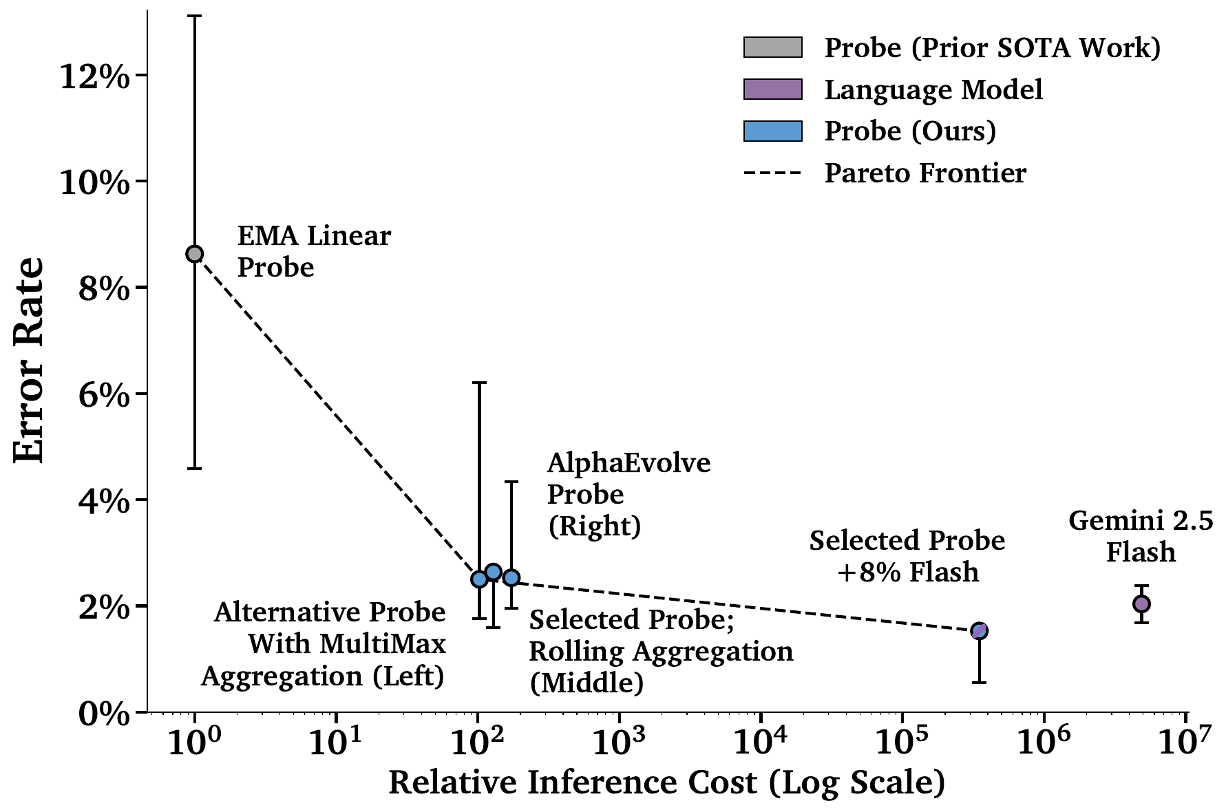
AlphaEvolve probes let an AI system search about 2,500 candidate combine steps, seeded from the attention probe. It rediscovered max-style combining on its own and closed roughly half the gap between the attention baseline and a perfect probe.
The combine rules in NumPy on a toy 40-position document with the attack at positions 20 to 23; the rolling mean here is plain, without the paper's attention weights.
import numpy as np
rng = np.random.default_rng(0)
# 40 positions; 20 to 23 are the attack
s = rng.normal(-1.0, 0.5, 40)
s[20:24] = 3.0
linear = s.mean()
ema, run = [], 0.0
for s_i in s:
    run = 0.5 * s_i + 0.5 * run
    ema.append(run)
ema_score = max(ema)
# MultiMax: 4 heads x 40 positions
S = rng.normal(-1.0, 0.5, (4, 40))
multimax = S.max(axis=1).sum()
win = np.ones(10) / 10
means = np.convolve(s, win, "valid")
rolling = means.max()
linear, mean pooling: the attack is diluted by the other 36 positions (Section 5.1).ema_score: a running average, then its maximum (eq card in Section 5.2, line 1).rolling: average each 10-position window, keep the largest (eq card in Section 5.2, line 2).Every rule then adds a bias and applies the sigmoid, and the prompt is flagged when p reaches 0.5; the question is which rule keeps one attack sentence above that line.
The weights are learned from labeled prompts (Figure 13).
The training loop for the single-head max probe, in the style of the paper's section 2, with random stand-ins for the cached activations and labels.
import torch, torch.nn as nn
# cached block-8 acts, 64 prompts
acts = torch.randn(64, 50, 768)
y = torch.randint(0, 2, (64,)).float()
probe = nn.Linear(768, 1)
params = probe.parameters()
opt = torch.optim.AdamW(params)
loss_fn = nn.BCEWithLogitsLoss()
for epoch in range(1000):
    # (64, 50): score per position
    s = probe(acts).squeeze(-1)
    z = s.max(dim=1).values
    loss = loss_fn(z, y)
    opt.zero_grad()
    loss.backward()
opt.step()Linear layer holds w and b; BCEWithLogitsLoss applies the sigmoid inside the loss.One deliberate choice shapes everything that follows: the probes are trained only on short prompts. Training on long-context data costs about 22 times more, because million-token activation sets overflow accelerator (TPU) memory. So long contexts stay a pure test the probe never studied for.
The decision threshold is picked on a validation set (held-out prompts the probe did not train on) with false alarms weighted heaviest, because a monitor with too many gets switched off. The toy on this page flags at p = 0.5.
The probe is cheap and the big model is not, so the paper pairs them: the probe decides the clear cases alone, and the unsure middle goes to Gemini 2.5 Flash for a second opinion.
The cascade scores lower error than Flash alone at roughly 1/50th the inference cost. The best thresholds are a plain deterministic pair, because a randomized defense would hand attackers a best-of-N exploit (retry N times, keep the best outcome).
The activations come from a forward hook on the tapped block. This listing uses GPT-2 small, which has the toy's shape (12 blocks, width 768): save copies block 8's output for each prompt into cache, and the training loop in section 6 reads them from there.
import torch
from transformers import GPT2Model, GPT2Tokenizer
tok = GPT2Tokenizer.from_pretrained("gpt2")
model = GPT2Model.from_pretrained("gpt2")
model.eval()
cache = []

def save(module, inputs, output):
    # output[0]: (1, T, 768)
    cache.append(output[0].detach())

# block 8, counting from 1
blk = model.h[7]
hook = blk.register_forward_hook(save)
text = "help me debug this code"
ids = tok(text, return_tensors="pt")
with torch.no_grad():
    model(**ids)
hook.remove()
torch.no_grad(), so the cache holds no graph.The paper tests the probes on short prompts, long documents, multi-turn chats, and real jailbreaks. A probe alone costs over 10,000 times less than an LLM judge and makes fewer errors.
Probes trained only on short prompts are scored on long contexts they never saw, on two rates where lower is better: FNR (false negative rate, the fraction of real attacks missed, left axis) and FPR (false positive rate, the fraction of benign prompts falsely flagged, right axis).
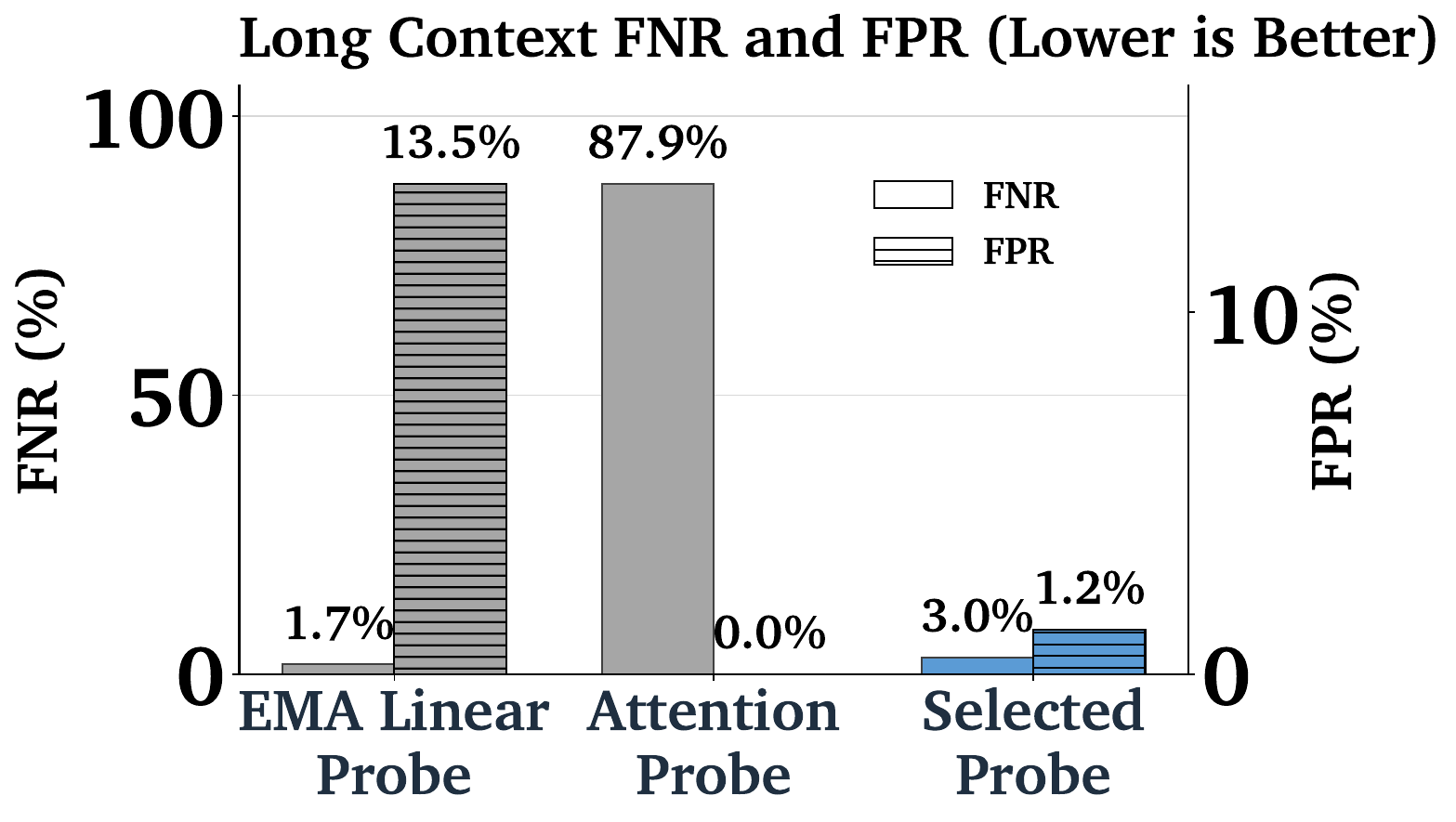
No single probe wins on every distribution shift (prompts in production differing in kind or length from the training prompts): the best one for long contexts is not the best for multi-turn chats, so each deployment picks its own.
Figure 19 puts the long-context trade-off on one plot. With no distribution shift at all, plain attention is already near-optimal.
Probes read a model's inner numbers to judge it. From BLIP to the Q-Former reads another model's inner numbers to feed a language model instead.